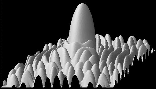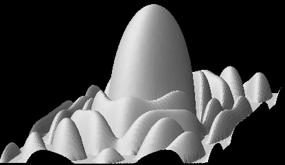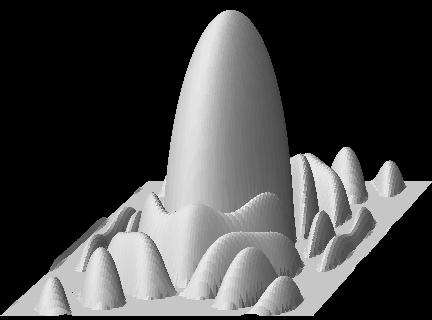
- Example SOLID-XYZ plot -
SOLID-XYZ produces wysiwyg (what-see-is-what-you-get) output for printing hardcopies, storing, and/or sharing plotted results. Output is available in PostScript and MIF (Maker Interchange Format) for importing graphs directly into a word-processor for documents, reports, and viewgraphs.
SOLID-XYZ supports automatic resizing of its window, and accepts a variety of input formats, including regular grid-spaced data, and arbitary 3-space data.

Blank lines are allowed anywhere in the file.
Example:
		0
		2
		1
		0
		next
		0
		0
		5
		0
		next
		0
		2
		2
		2
		next
		0
		2
		2
		2


The data are interpretted as follows:

		Z[ 0, 0 ]
		Z[ 1, 0 ]
		Z[ 2, 0 ]
		next
		Z[ 0, 1 ]
		Z[ 1, 1 ]
		Z[ 2, 1 ]
Where, Z[X,Y] represents the Z-value at row-X and column-Y in the grid (or matrix). On the display, the X-axis is drawn as the horizontal (left-to-right) axis. The Y-axis is drawn as the vertical (top-bottom) axis on the left of the screen. The Z-axis is represented for color-divisions on the graph with a color key on the right of the page.
By default, the X-and-Y axes take integer values corresponding to their row-column indices, from 0 to the number of points on the respective axis minus one. These can be renumbered by the 'replace_x_axis' and 'replace_y_axis' commands.
To render a smooth surface, the SOLID-XYZ-plotter interpolates randomly placed data-points onto a regular grid. The resolution of the grid defaults to 50x50. The 8-nearest neighboring points of your data are used to smoothly interpolate the value of each corresponding grid point. You can change the default grid resolutions and number of smoothing-points by the -xres, -yres, and -nsmooth command-line options.
Below is an example of x,y,z formatted data:
	     !      x          y	  z
		-1.645920   0.603504   0.054525
		-1.645920   0.201168   0.025225
		 1.280160   0.201168   0.052323
		 1.280160  -0.201168  -0.052323
		 0.182880   0.804672   0.238776
		 0.182880   0.402336   0.236319
		-1.645920  -0.201168  -0.025225
		-1.645920  -0.603504  -0.054525
Note that 'next' breaks are not needed with the explicit x,y,z format. One data point (x,y,z-tuplet) may be placed on each line of the data file. The data-points can occur in any order. Comments, axis-labels, and other commands may be interspersed on separate lines, as usual.
	Example,
		! Experiment Eight.
		!  (x,y,z)
		0
		2
		1
		next
		0
		5
		0
		next
		2
		2
		2
alias solidxyz '/home/bart/graph/solidxyz'Then type solidxyz with your data file specified on the command-line. For instance, to plot data in file f1.dat:
solidxyz f1.dat
Rotate Button - Allows you to select different angles of viewing
                perspective.  You can rotate the graph left-right
                and tilt it up-down.

ReDraw Button - Forces re-draw of the display.

ReSet Button - Resets all parameters to their initial defaults
		and then re-draws the display.

? Help Button - Causes a textual version of this help file to be displayed.

Print Button - Writes a postscript version of the plot as
		displayed to file called ljet.ps.  You can
		send the file file to a printer for hardcopy.

Quit Button - Quits the graph window.
Most display aspects can be changed interactively from the graph control-panel, so the command-line options are often more of a convenience. They enable the graph come up in a desired mode without pressing more buttons.
For non-interactive or script-driven usage, the command-line options are essential. They enable display modes to be set, or hardcopy print-outs to be generated, without the need of an interactive display for pressing buttons.
Below is a quick summary of the command-line options, followed by detailed descriptions of the important options.
	-ps	Non-Interactive PostScript output.  Useful for batch
		script-driven jobs.
	-mif	Non-Interactive MIF word-processor output.  Useful for
		batch script-driven jobs.
	-help	Prints this list of options.
	-x_range Specify X-axis range.  Must be followed by two values.
		If specified before files, used as Soft outer limits which
		will be stretched if data values exceed given range.
		If specified before files, used as Rigid range which will
		restrict graph boundaries even if data exceeds given range.
	-y_range Specify Rigid Y-axis range.  Must be followed by two values.
		If specified before files, used as Soft outer limits which
		will be stretched if data values exceed given range.
		If specified before files, used as Rigid range which will
		restrict graph boundaries even if data exceeds given range.
	-z_range Specify Z-axis range.  Must be followed by two values.
		If specified before files, used as Soft outer limits which
		will be stretched if data values exceed given range.
		If specified before files, used as Rigid range which will
		restrict graph boundaries even if data exceeds given range.
	-xres	Specify the x-axis resolution when using general x,y,z data.
	-yres	Specify the y-axis resolution when using general x,y,z data.
	-nsmooth Specify the number of neighboring points to use for
		interpolating general x,y,z data to the regular drawing grid.
	-ngrids_x - Specify number of horizontal axis grid tickmarks.
	-ngrids_y - Specify number of vertical axis grid tick-marks.
	-ngrids_z - Specify number of vertical axis grid tick-marks.
	-out_file - Specify postscript output file name.
	-lower_boundary - Position of lower graph border.
	-upper_boundary - Position of upper graph border.
	-left_boundary - Position of left graph border.
	-right_boundary - Position of right graph border.
Specify the horizontal axis range with:
-x_range min_x max_xwhere min_x and max_x are your desired range limits for the axis.
Specify the vertical axis range as in:
-y_range min_y max_ywhere min_y and max_y are your desired range limits for the axis.
Specify the Z-value range with:
-z_range min_z max_zwhere min_z and max_z are your desired range limits for the values.
You can use these to express 'hard' or 'soft' ranges. A 'hard' range means that the graph will be clipped exactly to the specified range, regardless of whether your data covers that range or exceeds it.
A 'soft' range means that the graph will be drawn out to that range even if your data does not span that range, but if data exists outside that range, the range will be extended to include the data.
You control the 'hardness' or 'softness' of your optionally specified ranges by where you place them on the command-line. If placed first on the command-line, the range specifier is 'soft' in that it acts merely as a minimum range. Any data coming afterward that exceeds that range will expand it. If placed last on the command line, the range specifier is 'hard' in that it sets the range to the specified value regardless of what the data range was that came before it.
The axes data ranges and their 'hardness' or 'softness' are independently controlled for the X, Y, and Z axes. For instance, you can specifiy the X-axis range, but let the Y- and Z-axes auto-scale to the data, by simply specifying only an X-axis range, or vice-verse.
If you are using SOLID-XYZ interactively, you can use the range specifiers to set the initial ranges. Then you can move around with the pan and zoom buttons, once you are inside the graph.
On command line: -upper_boundarywhere the-lower_boundary -left_boundary -right_boundary In file: upper_boundary = lower_boundary = left_boundary = right_boundary =
  Example:

	-ngrids_x 8
Will attempt to divide the axis into 8 tick-marks. The default values are: ngrids_x = 5, ngrids_y = 7, ngrids_z = 10.
title_x =You can turn the titles off by invoking SOLID-XYZ with the '-titles' option ahead of the graph name on the command line. The -titles option has a toggling affect, as do most of the other options, so you can turn it on-and-off several times across the command line to plot each file with different options. Specifying -titles a second time on the command line will turn the title sensitivity back on. This allows you select which files to include titles from when you are superimposing several files.title_y = title = Examples: title_x = Time (uS) This will put 'Time (uS)' under the X-axis. title_y = Device Name This will put 'Device Name' to the left of the Y-axis. title = Experiment 5: Two Search-mode Subgraphs. This will put 'Experiment 5: Two Search-mode Subgraphs.' across the top of the graph page.
  Example 1:

       solidxyz  -titles  f1.dat

     (This will only take titles from the f2.dat file.)
Sometimes it is convenient to have a dedicated file,
that have nothing but the common titles you like to use as in:
solidxyz result.dat velocity_graph.titles
The form is: annotationThe X-Y coordinate data are in the same coordinate system as your data (in other words, its not screen-coordinates, but data-coords.). The coordinate refers to the bottom left-hand corner of the text string.For example: anno 5.2 78.0 Second Experiment Results
To suppress annotations from appearing on you graph, you can use the '-sann', 'suppress annotations' command line option, or hit the Toggle-Annot button on the control panel.
To use this option, add the '-text' command-line. You embed text within your data file(s), by using the keyword 'text' followed by the inch-based coordinates of where you want it to appear on an 8.5x11 page. Then place your text on the succeeding lines. End the text entries by placing the keyword 'end_text' on an empty line. As with all other things, the keywords can be in caps or smalls or any combination thereof. An example follows:
	! This is an example of embedding text within a data file.
	! you might have axis titles and other things in here too.
	TEXT  4.5  3.2
	 Figure 8 - Revenue vs. Profits
	 	This text will be included on the graph
		when you select the '-text' option.
	END_TEXT
	! The data may then follow or precede the text, etc.
Command Syntax: replace_y_axisExample: replace_y_axis 101.2 VME_bus Action: The word 'VME_bus' will appear at the vertical position corresponding to 101.2 to the left of the y-axis where the numbers would otherwise appear.
Command Syntax: replace_x_axisExample: replace_x_axis 11 /device_11 Action: The word '/device_11' will appear at the horizontal position corresponding to 11 under the x-axis where the x-axis numbers would otherwise appear.
If you are not in interactive mode, invoke SOLID-XYZ with the '-ps' command-line option. A message will be printed to the screen saying that file 'ljet.ps' was written. To send it to a printer for hardcopy, type:
lpr ljet.psFile name 'ljet.ps' is the default output file name. You can specify a different name by using the -out_file command line option upon invocation, as in:
-out_file graph_3.psPostscript output would go to file 'graph_3.ps' instead of 'ljet.ps'.
You can then import the plot.mif file to your word-processor where you are free to manipulate the graph objects in any way that you choose. For instance, you can change fonts, font sizes, colors, etc.. You can also add textual annotations, with arrows to point to things, or circle or high-light particular graph features. One particularly powerful feature is the ability to stretch or shrink the whole graph, to change its aspect-ratio, or even rotate it 90-degrees. In this way you can easily put several graphs on a page with complete layout freedom.
File name 'plot.mif' is the default output file name. You can specify a different name by using the -out_file command line option upon invocation, as in:
-out_file graph_3.mifMIF output would go to file 'graph_3.mif' instead of 'plot.mif'.


Download alpha versions:
  For PC Linux:
   plot3d_101800.tar
  For Sun Solaris:
   plot3d_sun.tar
(Disclaimer: These versions are not very mature.)
Note: These are dynamically linked, which means that you must have the Motif run-time library (libXm.so). This is usually already part of most Solaris installations and is stable.
Linux installations may not include Motif, such as RedHat distributions prior to 7.3. Also your LD_LIBRARY_PATH variable must reference the Motif/lib, which is normally /usr/X11R6/lib/libXm.so.xx. If you do not have it, versions are available from www.opengroup.org/openmotif or www.lesstif.org, on "Powerware" disk of Redhat as RPM and other Linux distributions.
The present plot3d_101800.tar for Linux was compiled under Redhat 6.2 (kernel 2.2). It is known to work up to RedHat 7.2. For some reason backward compatibility seems to break at RedHat 7.3 and upward. We are looking at the situation. We may either provide a statically linked version, or a separate version for newer Linux's.
Please report comments, problems, or suggestions to :
 xgraphadmin@xgraph.org .

3-15-1999
See also:
